Wave energy analysis

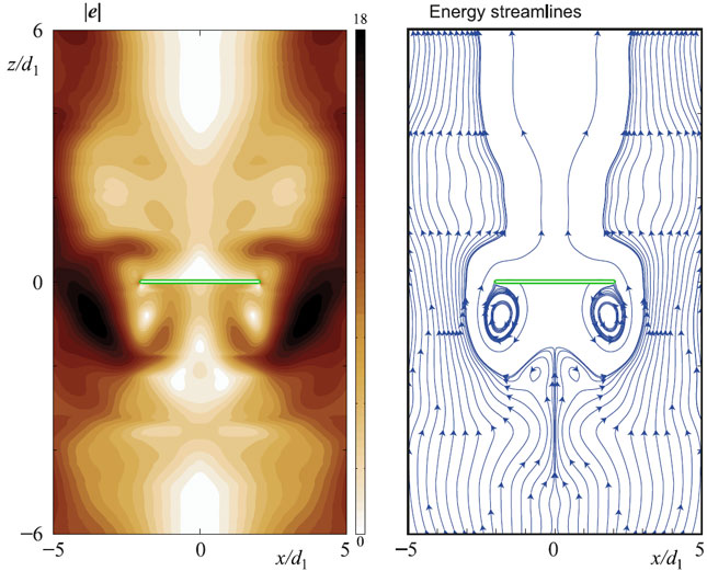
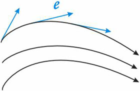
The transport of wave energy in the time-harmonic field can be visualized by the energy streamlines, which show the trajectories of time-averaged energy fluxes. At every point energy streamlines are tangential to the power density vector introduced by Umov for elastodynamic fields in 19th century. Its components can be calculated via the displacement and stress representations. Analysis of energy distribution gives deep insight into physics, it is sufficient for investigation of resonance phenomena and localization, especially scattering on inhomogeneities.

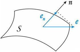
A time-averaged energy flux E across a surface S in the time-harmonic elastic wave field u(x) is introduced as an integral of the normal to S component of the averaged power density vector (Umov-Poynting vector) e(x) over S:

Averaged power density vector is calculated as scalar product of displacement and stress vectors:

while n is the unit outward normal for S. Continuous vector field e(x) determines in the space x a set of noncrossing curves x(s) to which e(s) is tangential at any point.

It has been known that there exist zones in the time-averaged energy flows in which the streamlines are closed. Centers of these zones, named energy vortices, are points of wavefront dislocations at which e=0.

Some examples are given below:

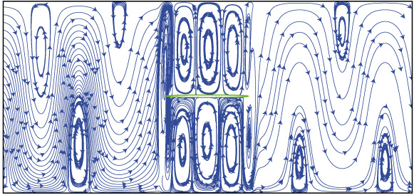
Energy flow corresponding to resonance motion of an elastic layer with a single strip-like crack

Energy flow in elastic phoninic crystal with a single strip-like crack in the middle of layer